\[ \DeclareMathOperator{\dexp}{dexp} \DeclareMathOperator{\ad}{ad} \]

Quantum Dynamics Simulation

A quantum computer is typically implemented via a set of controllable Hamiltonians. E.g.:

\[ H(t) = H_d + \sum_k a_k(t) H_k \]

where \(H_d\) is a drift Hamiltonian, \(H_k\) are a set on controllable (typically 2 to 3) Hamiltonians that are scaled by time-dependent parameter \(a_k(t)\). The goal is to find \(a_k(t)\) such that the system is driven to a desired unitary. The problem can be framed as a non-linear optimization problem by using the gradients (of error) of the time-evolution to find minima. Hence, the time-dependent Schrödinger equation needs to be solved, and the gradients of error for each \(a_k(t)\) need to be computed. In this chapter we look into the first part: how to solve the time-dependent Schrödinger equation.

The Objective

We want to find the propagator \(U(t, t_0)\) that connects the quantum state at different times,

\[ \ket{\psi(t)} = U(t, t_0)\ket{\psi(t_0)}. \]

The solution is often writen as

\[ U(t, t_0)=\mathcal T\exp\left[-i\int_{t_0}^tH(\tau)d\tau\right] \]

where \(\mathcal T\) is the time-ordering operator (see also Dyson series). But how does one numerically solve this? The standard treatment is to discretize the integrals as Riemann sums

(4)\[ U(t)\approx\prod_{a=0}^{k-1}\exp[-iH(a\Delta\tau)\Delta\tau]~~~~(\Delta\tau=t/k) \]

Note

Although this method is used in simulating quantum systems on classical computers, this technique is also commonly found in quantum computing literature with regards to implementating an operator \(U(t)\) as a quantum algorithm.

Equation (4) has given us a way to compute the propogator. However, a straightfoward analysis of this equation will show that the expansion is not unitary when truncated to finite order. Is this a better strategy to solve the time-dependent equation?

The following walks through the Magnus expansion, and solving the time-dependent Schrödinger equation when \(H\) does not commute with itself at different times, i.e. when \([H(t_1), H(t_2)] \neq 0\). The Magnus expansion conserves phase-space relationships. This means that energy is conserved even for long-time dynamics, where as other methods begin to fail – and thus the result remains unitary even when truncated.

For a thorough review: arXiv:0810.5488

Magnus Expansion

Consider the linear differential equation of the form

(5)\[ \begin{equation} Y^\prime(t) = H(t) Y(t);\quad Y(0) = Y_0 \end{equation} \]

whose solution can be expressed as

(6)\[ \begin{equation}\label{eq: sol} Y(t) = \exp(\Omega(t))Y_0 \end{equation} \]

where the difficulty lies in finding \(\Omega(t)\). Differentiating (6) results in:

(7)\[ \begin{equation}\label{eq: expansion} Y^\prime(t) = {d\over dt}\exp(\Omega(t))Y_0 = \dexp_{\Omega(t)}(\Omega^\prime(t))\exp(\Omega(t))Y_0 \end{equation} \]

where the derivative of the exponential map \(\dexp\) is defined as

\[ \begin{equation} \dexp_\Omega(C) = \sum_{i=0}^\infty \frac{1}{(i + 1)!}\ad_\Omega^i (C) \end{equation} \]

The operator \(\ad_\Omega^i(C)\) is the iterated commutator and recursively defined as:

\[ \ad_\Omega^i (C) = [\Omega, \ad_\Omega^{i-1}(C)], \quad i\ge 1 \]

Combining (5) and (7) leads to

\[ \begin{equation} H(t) = \dexp_{\Omega(t)} (\Omega^\prime(t)), \quad \Omega(0) = 0 \end{equation} \]

The inverse of the derivative of the exponential map will give

\[ \begin{equation} \Omega^\prime(t) = \dexp_{\Omega(t)}^{-1} (A(t)) \end{equation} \]

which is given by

\[ \begin{equation} \dexp_\Omega^{-1}(A) = \sum_{i=0}^\infty \frac{B_k}{k!}\ad_\Omega^i(A). \end{equation} \]

Here \(B_k\) are the Bernoulli numbers. The series converges only if

\[ \begin{equation} \int_0^t ||H(s)||_2 ds < \pi \end{equation} \]

By applying Picard’s Iteration, one gets an infinite series for \(\Omega(t)\):

\[ \begin{equation} \Omega(t) = \sum_{k=1}^\infty \Omega_k(t) \end{equation} \]

Where the first terms are:

\[\begin{split} \begin{align} \Omega_1(t) &= \int_0^t H(t_1) dt_1\\ \Omega_2(t) &= \frac{1}{2}\int_0^t dt_1 \int_0^{t_1} dt_2 [H(t_1), H(t_2)]\\ \Omega_3(t) &= \frac{1}{6}\int_0^t dt_1 \int_0^{t_1} dt_2 \int_0^{t_2} dt_3 ([H(t_1), [H(t_2), H(t_3)]] + [H(t_3), [H(t_2), H(t_1)]])\\ \end{align} \end{split}\]

Each subsequent order in the Magnus expansion is a correction that accounts for the proper time-ordering of the Hamiltonian.

Numerical Calculation

Assume a constant time step of size \(\Delta t\), thus the solution after one time step is

\[ \begin{equation} Y(t_n + \delta t) = \exp(\Omega(t_n + \delta t)) Y(t_n) \end{equation} \]

and hence

\[ \begin{equation} Y_{n+1} = \exp(\Omega_n) Y_n \end{equation} \]

First Order

To begin, truncate the series leaving only the first term, and approximate the integral with a Riemann sum. Hence,

\[ \Omega_n(\Delta t) = \Delta t H\left(t_n\right) \]

as an approximation for \(\Omega(t_n + \Delta t)\)

So the full approximation is

\[ Y_{n+1} = \exp(\Delta t H\left(t_n\right)) Y_n \]

Second Order

Truncate the series to the second term. Approximate the integral with a Gauss Quadrature. The approximation is then

\[ Y_{n+1} = \exp(\frac{\Delta t}{2}(A_1 + A_2) + \frac{\sqrt{3}\Delta t^2}{12}[A_2, A_1]) Y_n \]

where \(A_1 = A(t_n + c_- \Delta t)\) and \(A_2 = A(t_n + c_+ \Delta t)\) with \(c_\pm = \frac{1}{2}\pm \frac{\sqrt{3}}{6}\).

Python Example

As an example, let us simulate a simple quantum system

\[ H(t) = a(t)\sigma_x + a(t)\sigma_y \]

where \(a(t)\) is a Gaussian pulse. Particulary, we wish to see how the system involves in time. Let us also compare with the simulation performed by qutip.

import numpy as np
import qutip as qp
from scipy.linalg import expm
import matplotlib.pyplot as plt

X = np.array([[0, 1], [1, 0]])
Y = np.array([[0, 1j], [-1j, 0]])

print(X)
print(Y)

[[0 1]
 [1 0]]
[[ 0.+0.j  0.+1.j]
 [-0.-1.j  0.+0.j]]

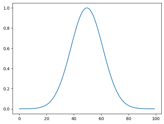
Create the pulse

t_r = np.linspace(0, 40, 100)

x = np.linspace(-3, 3, len(t_r))
pulse = np.exp(-x**2)
plt.plot(pulse)

plt.show()

Use QuTip to solve the evolution

H_qp = [[qp.Qobj(X), pulse], [qp.Qobj(Y), pulse]]
# H_qp = qp.Qobj(X)
psi = qp.basis(2,0)
result = qp.sesolve(H_qp, psi, t_r)

Use First-order Magnus Expansion

dt = t_r[1] - t_r[0]
dt

0.40404040404040403

psi_history = []

psi = np.array([[1], [0]])

for i in range(len(t_r)):
    Omega = dt * (pulse[i] * X + pulse[i] * Y)
    prop = expm(-1j * Omega)
    psi_history.append(psi)
    psi = prop @ psi

qp_evolution = np.array([s.full() for s in result.states])
magnus_1_evolution = np.array(psi_history)

plt.plot(qp_evolution[:, 0].real, color='r', label='Qutip')
plt.plot(qp_evolution[:, 0].imag, color='r')
plt.plot(qp_evolution[:, 1].real, color='r')
plt.plot(qp_evolution[:, 1].imag, color='r')

plt.plot(magnus_1_evolution[:, 0].real, '--', color='b', label='1st Order')
plt.plot(magnus_1_evolution[:, 0].imag, '--', color='b')
plt.plot(magnus_1_evolution[:, 1].real, '--', color='b')
plt.plot(magnus_1_evolution[:, 1].imag, '--', color='b')

plt.legend()

plt.title(r"1st Order with $\Delta t = {:.2f}$".format(dt))

plt.plot();

Use two-stage Gauss quadrature for second order

psi_history_2 = []

psi = np.array([[1], [0]])

c_1 = 0.5 - np.sqrt(3)/6
c_2 = 0.5 + np.sqrt(3)/6

def commu(A,B):
    return A@B - B@A

for i in range(len(t_r)):
    t_1 = x[i] + (c_1 * dt)
    t_2 = x[i] + c_2 * dt

    A_1 = np.exp(-t_1**2) * X + np.exp(-t_1**2) * Y
    A_2 = np.exp(-t_2**2) * X + np.exp(-t_2**2) * Y
    Omega = dt/2 * (A_1 + A_2) + np.sqrt(3)*dt**2 / 12 * commu(A_2, A_1)

    prop = expm(-1j * Omega)
    psi_history_2.append(psi)
    psi = prop @ psi

magnus_2_evolution = np.array(psi_history_2)

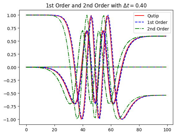
plt.plot(qp_evolution[:, 0].real, color='r', label='Qutip')
plt.plot(qp_evolution[:, 0].imag, color='r')
plt.plot(qp_evolution[:, 1].real, color='r')
plt.plot(qp_evolution[:, 1].imag, color='r')

plt.plot(magnus_1_evolution[:, 0].real, '--', color='b', label='1st Order')
plt.plot(magnus_1_evolution[:, 0].imag, '--', color='b')
plt.plot(magnus_1_evolution[:, 1].real, '--', color='b')
plt.plot(magnus_1_evolution[:, 1].imag, '--', color='b')

plt.plot(magnus_2_evolution[:, 0].real, '-.', color='g', label='2nd Order')
plt.plot(magnus_2_evolution[:, 0].imag, '-.', color='g')
plt.plot(magnus_2_evolution[:, 1].real, '-.', color='g')
plt.plot(magnus_2_evolution[:, 1].imag, '-.', color='g')

plt.legend()

plt.title(r"1st Order and 2nd Order with $\Delta t = {:.2f}$".format(dt))

plt.show()