Randomness
Contents
Randomness#
Measure theory studies things that are measurable (e.g. length, area, volume) but generalized to various dimensions. The measure tells us how things are distributed and concentrated in a mathematical space.
Example: The Sphere
Any point on the sphere can be specified by three parameters: e.g. (x,y,z) in Cartesian coordinates or \((\rho, \theta, \phi)\) in spherical coordinates.
Suppose we wish to find the volume. The first thought may be to integrate each parameter over its full range:
But this is clearly wrong (the volume of a sphere with radius \(r\) is \(\frac{4}{3}\pi r^3\).) Taking the integral in this way does not account for the structure of the sphere with respect to the parameters. If you have ever studied multivariate calculus this may sound familiar.
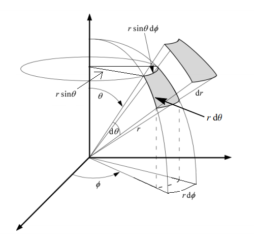
The issue is that although the difference \(d\theta\) and \(d\phi\) are the same, there is more stuff near the equator of the sphere. Therefore the integral must account for the value of \(\theta\). Similarly, as we are closer to the center of the sphere there is less stuff compared to as we go further away from the center. Hence we must also include the radius \(\rho\) as part of the integral.
So the correct integral is:
The extra terms \(\rho^2\sin\theta\) is the measure. The measure weight portions of the sphere differently depending on where they are in the sphere.
Although the measure tells us how to properly integrate, is also tells us another important fact: how to sample points in the spae uniformly as random. We cannot simply take each parameter and sample it from the uniform distribution – this does not take into account the spread of the space. The measure tells us the distribution of each parameters and let us obtain something truly uniform.
Haar Measure#
Quantum evolutions (and operations in quantum computing) are described by unitary matrices. Just like the sphere, unitary matrices can be expressed in terms of a fixed set of parameters. For example, a qubit operation can be written as:
where \(v_x^2 + v_y^2 + v_z^2 = 1\). We ignore \(e^{i\alpha}\) because it is a global phase. So we are left with four parameters. But because we have the constraint that \(v_x^2 + v_y^2 + v_z^2 = 1\), we only need a total of 3 parameters to describe a single qubit operation.
In fact we can write any unitary matrix (ignoring global phase) of size \(N \times N\) as:
where \(\vec{\Lambda}\) contains \(N^2 -1\) traceless Hermitian operators that define space, similar to the Pauli matrices for the case \(N=2\).
For a dimension \(N\), the unitary matrix of size \(N \times N\) form the unitary group \(U(N)\).
Note
Because we ignored the global phase, the operations we provided are technically \(SU(N)\) the special unitary group, where \(det(U) = 1\).
Just like the points of the sphere, we can perform operations on the unitary group: such as integration, functions, and sample uniformly. But just like the sphere, we have to add the measure in order to properly account for the different weights in different regions of the space. This is known as the Haar measure, is often denoted as \(\mu_N\).
\(\mu_N\) tells us how to weight the elements of \(U(N)\). So for example, if we have some function \(f\) acting on the elements of \(U(N)\) and we would like to integrate over this group, we would have:
Example: qubit#
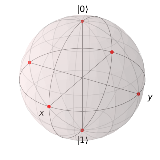
Let us consider the following task: generate a random qubit state. To do this let us generate a Haar-random unitary and then apply it an initial state (e.g. \(\ket{0}\)).
First let us do this incorrectly. To make things easier, let us use the following representation of a single-qubit gate:
def bad_random_qubit_unitary():
    phi, theta, lam = 2 * np.pi * np.random.uniform(size=3)
    U = np.array([
            [np.cos(theta/2), -np.exp(-1j * lam) * np.sin(theta/2)],
            [np.exp(1j * phi) * np.sin(theta/2), np.exp(1j * (phi + lam) * np.cos(theta/2))]
        ])
    return U

samples = 1000

bad_random_unitaries = [bad_random_qubit_unitary() for _ in range(samples)]
bad_random_states = [U[:,0] for U in bad_random_unitaries]
states = [qp.Qobj(s) for s in bad_random_states]
b = qp.Bloch()
b.point_color = ['#ff0000']
b.point_marker = ['o']
b.add_states(states, kind='point')
b.show()
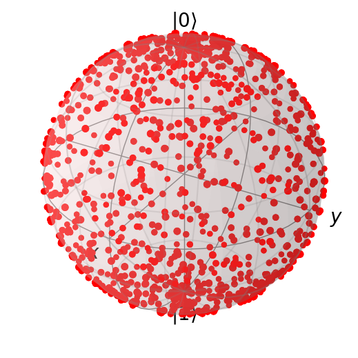
Note that although we uniformly sampled our parameters, the output states cluster around the poles of the sphere. Now let us properly sample from the proper Haar measure.
Unlike the regular sphere, our sphere has a fixed radius of 1, so we need not worry about this parameter. However, similar to the regular sphere, we need to worry about \(\theta\). Since the adjustment is identical to the regular sphere, we can use \(\sin\theta\). Hence, in order to uniformly sample \(\theta\) we need to use the distribution \(\mathrm{Pr}(\theta) = \sin \theta\).
from scipy.stats import rv_continuous

class sin_theta_dist(rv_continuous):
    def _pdf(self, theta):
        return 0.5 * np.sin(theta)

sin_theta_sampler = sin_theta_dist(a=0, b=np.pi)

def haar_random_qubit_unitary():
    phi, lam = 2 * np.pi * np.random.uniform(size=2)
    theta = sin_theta_sampler.rvs(size=1)
    U = np.array([
        [np.cos(theta/2), -np.exp(-1j * lam) * np.sin(theta/2)],
        [np.exp(1j * phi) * np.sin(theta/2), np.exp(1j * (phi + lam) * np.cos(theta/2))]
    ])
    return U

haar_random_unitaries = [haar_random_qubit_unitary() for _ in range(samples)]
haar_random_states = [U[:,0] for U in haar_random_unitaries]
states = [qp.Qobj(s) for s in haar_random_states]
b = qp.Bloch()
b.point_color = ['#ff0000']
b.point_marker = ['o']
b.add_states(states, kind='point')
b.show()
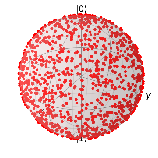
As we can see, by using the correct measure, our qubit states are now uniformly distributed over the sphere. Explicitly, our Haar measure is:
Example: arbitrary dimension#
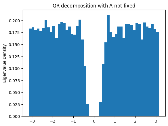
Following arXiv:math-ph/0609050, we can use the QR decomposition of a complex-valued matrix to generate Haar-random unitary matrices. This actually implemented in scipy.stats.unitary_group.
def haar_random_unitary(N, fixed=True):
    R, I = np.random.normal(size=(N,N)), np.random.normal(size=(N,N))
    Z = R + 1j * I

    Q, R = np.linalg.qr(Z)

    if fixed:
        L = np.diag([R[i, i] / np.abs(R[i, i]) for i in range(N)])
        Q = Q @ L

    return Q

N = 10
rand = [haar_random_unitary(N) for _ in range(samples)]
rand_not_fixed = [haar_random_unitary(N, fixed=False) for _ in range(samples)]
As explained in arXiv:math-ph/0609050, the solution to the QR decomposition is not unique. We can take any unitary diagonal matrix \(\Lambda\), and alter the decomposition as \(QR = Q \Lambda \Lambda^\dagger R = Q^\prime R^\prime\). To insure the unitary matrices are indeed Haar-random, we need to fix a particular \(\Lambda\) which depends on \(R\).
Another fact is that the eigenvalues of a Haar-random unitary matrices should be uniform. And the eigenvalues of a unitary matrix are given as \(e^{i\theta}\). Let us check that using the QR-decomposition method our \(\theta\) eigenvalues are indeed uniform.
eigs_rand = np.array([np.linalg.eigvals(r) for r in rand_not_fixed]).flatten()

hist = plt.hist(np.angle(eigs_rand), 50, density=True)
plt.ylabel("Eigenvalue Density")
plt.title(r"QR decomposition with $\Lambda$ not fixed")
plt.show()
eigs_rand = np.array([np.linalg.eigvals(r) for r in rand]).flatten()

hist = plt.hist(np.angle(eigs_rand), 50, density=True)
plt.ylabel("Eigenvalue Density")
plt.title(r"QR decomposition with $\Lambda$ fixed")
plt.show()
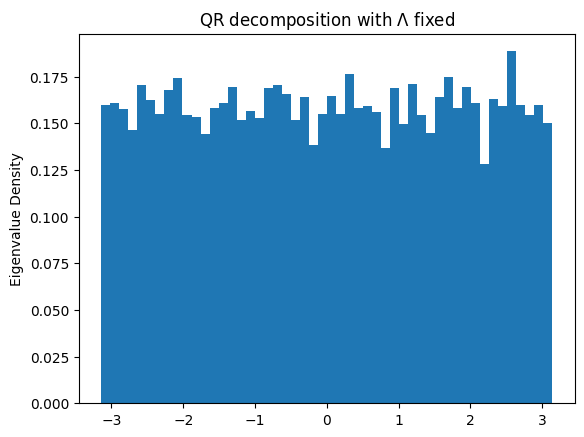
We have successfully generated Haar-random unitary matrices as shown by the uniform distribution of their eigenvalues.
Twirling#
Important
Twirling a quantum channel \(\mathcal{E}\) consists of averaging \(\mathcal{E}\) under the composition \(\mathcal{U} \circ \mathcal{E} \circ \mathcal{U}^\dagger\) for unitary operations \(U(\rho) = U \rho U^\dagger\) chosen according to some probability distribution. The average channel
is known as the twirled channel.
When the distribution over unitaries is discrete we have
Sampling from the uniform Haar-measure \(\mu_N\), (2) becomes
Intuitively, because all the elements are from the full unitary group, we would expect that the resulting channel contains a large amount of symmetry lettings us describe with it a small number of parameters. And indeed! The resulting operation can be described as the depolarizing channel
where \(p \in [0, 1]\).
Average Gate Fidelity#
In many instances it is useful to estimate how “close” a quantum operation is to a given unitary operation. For instance during a quantum computation one may want to implement the unitary gate \(U\) and, as with any physical implementation, this will not be perfect. Thus the resulting operation will be represented by a channel \(\mathcal{E}\). It would be useful to have an idea of how well \(\mathcal{E}\) approximates \(\mathcal{U}\). As noted previously there are many different measures of how close two quantum operations (e.g. the fidelity and trace distance). One important measure is related to the fidelity and is called the average gate fidelity.
The average gate fidelity between \(\mathcal{E}\) and \(\mathcal{U}\), \(\overline{{{F_{g}}}}({\mathcal E},\mathcal U)\) is given by
The integral is over the unitarily Fubini-Study measure on pure states. We can rewrite this expression as
where \(\Lambda\) is the cumulative noise operator
and \(U\) is the unitary Kraus operator for \(\mathcal{U}\).
If we twirl \(\Lambda\) we can then write
As derived in arXiv:quant-ph/0205035, we can express this as
where \(\{ A_k \}\) are a set of Kraus operators for \(\mathcal{E}\).
p is called the noise strength parameter and characterizes how well \(\mathcal{E}\) approxi- mates \mathcal{U}. If \(p\) is close to 1, then \(\mathcal{E}\) approximates \(\mathcal{U}\) well, while if p is close to 0 then \(\mathcal{E}\) does not resemble \(\mathcal{U}\).
The Protocol#
Let us now express the protocol for estimating \(\overline{{{F_{g}}}}(\mathcal{E}, \mathcal{U})\).
We have
which is the average over the unitary group of the function \(f : U(N) \mapsto \mathbb{R}\) defined by
\(\rho\) may be taken as the computation basis \(\ket{0} ... \ket{0}\ket{0}\bra{0}...\bra{0}\bra{0}\). This essentially tells us that if choose a unitary operator at random and implement it, then \(f(U)\) will be close to the average \(\overline{{{F_{g}}}}({\mathcal{E}},{\cal{U}})\) in that
Caution
There are two main drawbacks to this protocol for the determining the average fidelity of \(\mathcal{E}\) and U,
Choosing a random unitary over the Haar measure is exponentially hard in system dimension \(N\).
Infeasible in general, to calculate \(f(U)\) for a unitary \(U\), one needs to either
perform a measurement in the basis defined by \(U\) acting on the computational basis
or perform full process tomography on the output \(\mathcal{E}(\rho) = \Lambda \circ \cal{U}(\rho)\)
t-designs#
Let us see how we can overcome the drawbacks described above. However, before doing so, let us consider a sphere for intuition.
Suppose we have a polynomial of \(d\)-variables, and we seek to compute the average of the polynomial over a \(d\)-dimensional unit sphere. However, this comes with some difficulty:
Integrate the polynomial over the sphere, using a proper measure – but keeping track of all the parameters is difficult
Approximate the average value by sampling points of the sphere uniformly, computing the function value at those points, and then average them – but this only an approximation.
Fortunately, there a nice theorem that tells us if the terms in the polynomial have the same degree of at most \(t\), then we can compute the average exactly over the sphere using only a number of points. The set of points that give us the result is called a spherical t-design.
Mathematically, let \(p_t\) be a polynomial in \(d\) variables, with all terms the same degree of at most \(t\). A set \(X\) is a spherical t-design if
holds for all possible \(p_t\), where \(d\mu\) is the uniform spherical measure. A spherical t-design is also a k-design for all \(k<t\).
Example: The Sphere#
Let us find the average of the polynomial
over our unit sphere. Because all the terms in the polynomial have degree of 2, we can approximate the average by using a 2-design which happens to be a pyramid. However, let use a 3-design (a cube) for convenience – it still forms a 2-design.
cube = np.array([
    [1, 1, 1], [1, 1, -1], [1, -1, 1], [1, -1, -1],
    [-1, 1, 1], [-1, 1, -1], [-1, -1, 1], [-1, -1, -1],
])

# normalize to make sure point is in the unit sphere
cube = np.array([p / np.linalg.norm(p) for p in cube])
Now, let us calculate the average
def f(x,y,z):
    return x**2 + x * y - x * z

avg = np.mean([f(*p) for p in cube])
print(avg)
0.3333333333333334
Now let us extend our definitions so far to unitary matrices. A unitary design utilize evenly-distributed unitaries to average polynomials that are functions of entries of unitary matrices.
Mathematically, let \(p_{t,t}\) be a polynomial where the \(d\) variables are the entries of a unitary matrix \(U\) such that they have the same degree of at most \(t\). Moreover, the complex conjugate of those entries must also be the same degree \(t\). A unitary \(t\)-design is a set of \(K\) unitaries \(\{U_k\}\) such that
holds for all possible \(P_{t,t}\) and where \(d\mu\) is the uniform Haar measure.
There exists a unitary design for all possible combinations of \(t\) and \(d\). For example, a 2-design in dimension \(d\) has at least \(d^4 - 2d^2 + 2\) elements. But finding these sets (and ones with minimal size) is a challenging problem, but some recent constructions have been made. The most commonly used unitary design is perhaps the 2-design.
Average Fidelity#
Suppose we have a noisy channel \(\cal{E}\), and our desired unitary operation \(U\). For simplicity let us suppose we start in an initial state \(\ket{0}\) and we apply Haar-random operators \(V\) to \(\ket{0}\) to get Haar-ransom states. The average fidelity:
This should look familiar – we have twirled the channel \(\cal{E}\). Let us look closely at this expression: we have an inner product involving two instances of \(V\) and two instances of \(V^\dagger\). The expression is a polynomial of degree 2 in both the elements of \(U\) and the complex conjugate! So if can find \(K\) unitaries that form a 2-design, we can compute the average fidelity
But should be our set of unitaries?
Clifford Group#
Turns out there are some groups that are unitary designs:
Pauli group is unitary 1-design
Clifford group is unitary 3-design (also 2-design and 1-design)
The n-qubit Pauli group, \(\cal{P}(n)\), is the set of all tensor products of Pauli operations X, Y, Z, and I. The n-qubit Clifford group, \(\cal{C}(n)\), is the normalizer of the Pauli group. In other words, the Clifford group is the set of operations that send Paulis to Paulis (up to a phase) under conjugation:
Clifford groups have many interesting properties and have countless of uses in quantum computing. For example, stabilizer circuits – composed of purely Clifford gates and measurement – can be efficiently simulated on a classical computer.
Clifford group is generated by three gates, Hadamard, S, and CNOT gates. For a single qubit the Clifford group contains 24 elements, and we can see that they are evenly distributed:
qubit_cliffords = [
    '',
    'H', 'S',
    'HS', 'SH', 'SS',
    'HSH', 'HSS', 'SHS', 'SSH', 'SSS',
    'HSHS', 'HSSH', 'HSSS', 'SHSS', 'SSHS',
    'HSHSS', 'HSSHS', 'SHSSH', 'SHSSS', 'SSHSS',
    'HSHSSH', 'HSHSSS', 'HSSHSS'
]

psi_0 = np.array([[1], [0]])

H = np.array([[1, 1], [1, -1]]) / np.sqrt(2)
S = np.array([[1, 0], [0, 1j]])

states = []

for c in qubit_cliffords:
    op = np.eye(2)
    for u in c:
        if u == 'H':
            op = op @ H
        elif u == 'S':
            op = op @ S
    state = qp.Qobj(op @ psi_0)
    states.append(state)

b = qp.Bloch()
b.point_color = ['#ff0000']
b.point_marker = ['o']
b.add_states(states, kind='point')
b.show()
Instead of using all Clifford group elements, modern approaches for randomized benchmarking use uniformly random Clifford operators.