Device Characterization
Contents
Device Characterization#
Quantum computers are real quantum systems that we wish to design and control. Moreover, quantum computers face quite the conflicting requirements: on one hand we wish to interact with the system to control and measure it; but on the other hand we wish to protect the system from the environment. None the less, experimental realizations of quantum computers has made significant progress in the past two decades.
Superconducting Qubits#
The Cooper Pair Box (CPB) Hamiltonian is:
where \(H_{el}\) is the electrostatic component and \(H_j\) is the nonlinear Josephson junction component. These can be written as:
where \(E_j\) is the Josephson energy of the junction, and \(E_c\) is the charging energy inversely proportional to the total capacitance of the qubit circuit.
This Hamiltonian is written in the basis of charge eigenstates, which is associated with the number \(\hat{n}\) of Cooper pairs.
As a matrix, the Hamiltonian looks like
The eigenvector relation
gives us
with boundary condition: \(\psi_0 = \psi_{r+1} = 0\).
The Hamiltonian in Phase Basis#
The operator conjugated to \(\hat{n}\) is the superconducting phase \(\hat{\theta}\):
where there is a circular topology:
The set \(\{|\theta\rangle, \theta \in [0, 2\pi]\}\) for a complete basis.
The \(\hat{\phi}\) is superconducing phase difference which satisfies the commutation relation with \(\hat{N}\):
In the phase representation the Hamiltonian can be written as:
Where \(\phi\) must satisfy boundary conditions: \(\phi(\theta) = \phi(\theta + 2\pi)\). This has the form of a Mathieu differential equation, which has known analytical solutions using Mathieu functions.
The eigenvalues are:
Fitting the Hamiltonian#
In reality, once a superconducting chip is built, we do not have access to what the values of \(E_j\) and \(E_c\) are and therefore we must recover them. What we do have access to the is frequencies (energies) of the qubit.
As a first step, we can approximate \(E_c\) and \(E_j\) using the first three transition frequencies
\(w_{01} = E_1 - E_0\)
\(w_{12} = E_2 - E_1\)
As an example, let us take the first free energy levels of ibmq_armonk and estimate \(E_c\) and \(E_j\):
freq = [4.80637   , 4.58210259, 4.33777661]
freq = np.array(freq)

E_c = (freq[0] - freq[1])
E_j = (freq[1] + E_c)**2/(8*E_c)
ng = 0

print(f"Approximation for E_c and E_j: {E_c}, {E_j}")
Approximation for E_c and E_j: 0.2242674100000004, 12.875919297023563
Optimizing the Fit#
Let us try to improve the fit by comparing how close the estimated energies are to the original energies, and then shifting the Hamiltonian parameters.
A helper class computes the Hamiltonian and frequency transitions of a Transmon
class Transmon:
    def __init__(self, n_cut=40):
        self.n_cut = n_cut
        self._n = np.diag(np.arange(-n_cut, n_cut + 1))
        self._hc_n2 = 4 * self._n @ self._n
        self._hc_n1 = -2 * 4 * self._n
        self._hc_n0 = 4 * np.eye(len(self._n))
        self._hj =  -.5 * (np.diag(np.ones(2 * n_cut), 1) + np.diag(np.ones(2 * n_cut), -1))

    def __call__(self, ec, ej, ng=0, grad=False, grad_includes_ng=False):
        h = ec * (self._hc_n2 + ng * self._hc_n1 + ng**2 * self._hc_n0) + ej * self._hj

        if grad:
            dh_dec = (self._hc_n2 + ng * self._hc_n1 + ng**2 * self._hc_n0)
            dh_dej = self._hj
            if grad_includes_ng:
                dh_dng = ec * (self._hc_n1 + 2 * ng * self._hc_n0)
                grads = np.stack([dh_dec, dh_dej, dh_dng], axis=0)
            else:
                grads = np.stack([dh_dec, dh_dej], axis=0)
            return h, grads
        return h

    def transitions(self, ec, ej, ng=0, grad=False, grad_includes_ng=False):
        if grad:
            h, grads = self(ec, ej, ng=ng, grad=grad, grad_includes_ng=grad_includes_ng)
            vals, vecs = np.linalg.eigh(h)
            d_vals = np.einsum('xij,ia,ja->xa', grads, vecs.conj(), vecs)
            return np.diff(vals), np.diff(d_vals, axis=-1)
        return np.diff(np.linalg.eigvalsh(self(ec, ej, ng=ng)))
Now let us optimize
def loss_with_grad(ec_ej_ng):
    t, dt = transmon.transitions(*ec_ej_ng, grad=True, grad_includes_ng=len(ec_ej_ng)==3)
    t = t[:freq.size]
    dt = dt[:, :freq.size]
    r = t - freq
    dr = dt
    loss = r @ r
    grad_loss = 2 * dr @ r
    return loss, grad_loss

transmon = Transmon(40)

x0 = [E_c, E_j, ng]

from scipy.optimize import minimize
result = minimize(loss_with_grad, x0=x0, jac=True)

print(f"Fitted E_c, E_j, and ng: {result.x}")
Fitted E_c, E_j, and ng: [ 2.01700138e-01 1.55999907e+01 -1.37202718e-14]
Error Landscape#
Let us visualize the error in different Hamiltonian parameters
ec, ej = x0[:2]
EJ = np.linspace(ej * (1 - .9), ej * (1 + .9), 51)
EC = np.linspace(ec * (1 - .9), ec * (1 + .9), 50)
losses = np.zeros((EC.size, EJ.size))
grads = np.zeros((EC.size, EJ.size, 2))
for i, ec in enumerate(EC):
    for j, ej in enumerate(EJ):
        losses[i, j], grads[i, j] = loss_with_grad([ec, ej])
plt.pcolormesh(EC, EJ, np.log(losses.T))
plt.plot(*x0[:2], 'rd', label="Approximation")
plt.plot(*result.x[:2], 'r*', label="Optimization")
plt.xlabel("E_c")
plt.ylabel("E_j")
plt.title("Error Landscape")
plt.colorbar()
plt.legend()
plt.show()
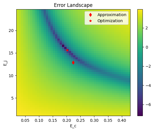
print(f"E_c/E_j: {result.x[0]/result.x[1]}")
E_c/E_j: 0.012929503687487498
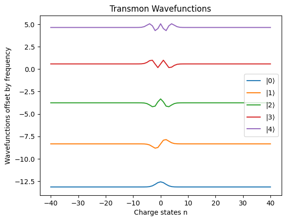
As a Qubit#
We can use the first two levels of the superconducting transmon to be our qubit. A key feature is that the energy levels are anharmonic, or in other words, the spacing between energy levels varies. This feature is crucial to be able to specifically control the qubit.
H = transmon(*result.x)

eigs, evecs = np.linalg.eigh(H)

plt.title("Transmon Wavefunctions")

x = range(-transmon.n_cut, transmon.n_cut+1)

plt.plot(x, evecs[:,0] + eigs[0], label=r"$|0\rangle$")
plt.plot(x, evecs[:,1] + eigs[1], label=r"$|1\rangle$")
plt.plot(x, evecs[:,2] + eigs[2], label=r"$|2\rangle$")
plt.plot(x, evecs[:,3] + eigs[3], label=r"$|3\rangle$")
plt.plot(x, evecs[:,4] + eigs[4], label=r"$|4\rangle$")
plt.xlabel("Charge states n")
plt.ylabel("Wavefunctions offset by frequency")
plt.legend()
plt.show()
References:
Lev Simon Bishop Thesis