Holonomic Quantum Computing
Contents
Holonomic Quantum Computing#
Why?#
Rely on stable topological features to produce unitary operators
The hope is that (in practice) the topological features provide more error tolerance
Loops in the control manifold can induce a unitary operator that depends on the area of the loop
Review of geometric phase via Adiabatic Evolution#
Consider
Let the system start in the eigenstate:
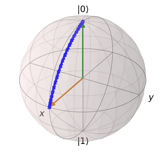
theta_0 = np.pi / 3 # we will keep theta constant
phi_0 = 0 # we will rotate phi

psi_0 = np.cos(theta_0/2) * qp.basis(2,0) + np.exp(1j * phi_0) * np.sin(theta_0/2) * qp.basis(2,1)

b = qp.Bloch()
b.add_states(psi_0)
b.show()
phi_f = 2*np.pi

tau = 2**10 * np.pi

def angle(t):
    return (1 - (t/tau))* phi_0 + (t/tau) * phi_f

H = [
    [qp.sigmax(), (lambda t, args: np.sin(theta_0) * np.cos(-angle(t)))],
    [qp.sigmay(), (lambda t, args: np.sin(theta_0) * np.sin(-angle(t)))],
    [qp.sigmaz(), (lambda t, args: np.cos(theta_0))]
]

t_range = np.linspace(0, tau, 100)

result = qp.mesolve(H, psi_0, t_range)
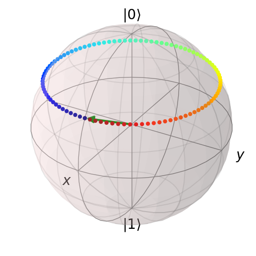
Our Hamiltonian is cyclic! \(H(\pi/3, 0) = H(\pi/3, 2\pi)\). Let us plot the \(B\) field along with initial state.
# plot the control

from matplotlib import cm, colors

nrm = colors.Normalize()
colors = cm.jet(nrm(t_range))

b.point_color = colors

b.add_points([np.sin(theta_0) * np.cos(-angle(t_range)), np.sin(theta_0) * np.sin(-angle(t_range)), [np.cos(theta_0) for _ in t_range]], 'm')

b.show()
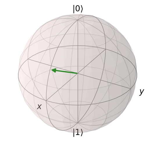
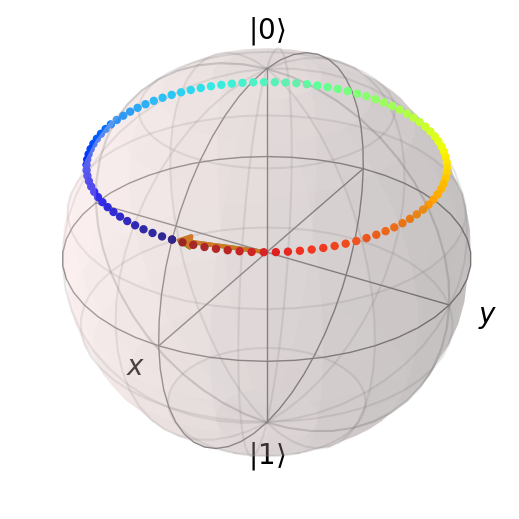
Let us plot the final state
b.add_states(result.states[-1])
b.show()
overlap = result.states[-1].overlap(psi_0)
print(f'State similarity: {np.abs(overlap)**2}')
State similarity: 0.9999992855589531
gamma = np.pi * (np.cos(theta_0) - 1)
expected = np.exp(1j * gamma)
print(f'Calculated {overlap}\nExpected {expected}')
Calculated (-0.0004978402668791111-0.9999995188568952j)
Expected (5.053215498074303e-16-1j)
The Math#
The eigenstate equation:
A general state can be written in terms of eignestates:
where
and is known as the dynamical phase.
By plugging the general state into the Schrondinger equation, we arrive at:
Assuming there is no degeneracy, one particular amplitude in the eigenbasis gives
If the Hamiltonian evolves slowly in time compared to the difference between energy level, then the second term goes away, which results in
where
This phase is known as Berry’s Phase.
Suppose the Hamiltonian’s time dependence can be described by a vector of parameters \(\mathbf{R}(t)\). Then the integrand from Berry’s phase can be written as:
So the integral can then be evaluated along a curve in parameter space
If the time evolution is cyclic, with period T such that \(\mathbf{R}(0)= \mathbf{R}(T)\), then by Stokes’ theorem:
where \(d\mathbf{a}\) is a vector of measures for each parameter.
Review of non-Abelian Generalization of Geometric Phase (holonomy)#
Holonomy refers to the set of closed curves starting and ending at some point, they form a group
The geometric phase is a abelian representation of an holonomy group – any loop is associated with a geometric phase factor and they commute: \(e^{i\gamma_1} e^{i\gamma_2} = e^{i\gamma_2}e^{i\gamma_1}\)
So a non-abelian generalization can be represented by matrices
Can be shown by inspecting a degenerate subspace subject to an adiabatic evolution
The Math (2)#
Previously, we made the assumption that there was no degeneracy. However, suppose our initial state belongs to a degenerate subspace. Then following the same treatment, the system will stay within the subspace. The time evolution of the coefficient will now include an additional sum:
The solution is now a matrix exponential
where \(T\) is the time-ordering operator.
In the case we have vectors, then we define
A unitary is then implemented in the subspace
Review of nonadiabatic Holonomic Quantum Computation#
Assume an \(N\)-dimensional quantum system subject to a Hamiltonian \(H(t)\)
Assume there is an \(L\)-dimensional subspace, \(S(t) = span\{|\phi_k\rangle\}_{k=1}^L\) where \(|\phi_k(t)\rangle\) are orthonormal vectors and satisfy the divine equation: \(i \frac{d}{dt}|\phi_k(t)\rangle = H(t)\phi_k(t)\rangle\)
There is a unitary operator \(U(\tau)\), \(|\phi_k(\tau)\rangle = U(\tau)|\phi_k(0)\rangle\), if \(|\phi_k(t)\rangle\) satisfy:
- \[\sum_{k=1}^L |\phi_k(\tau)\rangle\langle \phi_k(\tau)| = \sum_{k=1}^{L} |\phi_k(0)\rangle\langle \phi_k(0)|\]
- \[\langle \phi_k(t)| H(t) |\phi_l(t)\rangle = 0, \quad k,l = 1,...,L\]
Nonadiabatic Holonomic Qubit Gate (via 3 levels)#
Suppose the Hamiltonian (in the interaction picture) is:
import matplotlib.pyplot as plt

fig = plt.figure(figsize=(3, 5))
ax = fig.subplots()
line = np.arange(0,1,0.01)
ax.plot(line, 0 * line, c='black')
ax.plot(line, 1 + 0* line, c='black')
ax.plot(line, 1.6 + 0* line, c='black')

ax.annotate("",
            xy=(0.5, 0), xycoords='data',
            xytext=(0.5, 1), textcoords='data',
            horizontalalignment="center",
            arrowprops=dict(arrowstyle="<->",
                            color='blue',
                            lw=2),
            )
ax.annotate("",
            xy=(0.5, 1), xycoords='data',
            xytext=(0.5, 1.6), textcoords='data',
            arrowprops=dict(arrowstyle="<->",
                            color='green',
                            lw=2),
            )
ax.text(0.55, 0.5, r"$a\Omega(t)$", fontsize='large')
ax.text(0.55, 1.3, r"$b\Omega(t)$", fontsize='large')

ax.text(1.0, -0.015, r"$|0\rangle$", fontsize='large')
ax.text(1.0, 1 - 0.015, r"$|e\rangle$", fontsize='large')
ax.text(1.0, 1.6 - 0.015, r"$|1\rangle$", fontsize='large')

ax.axis('off')
plt.show()
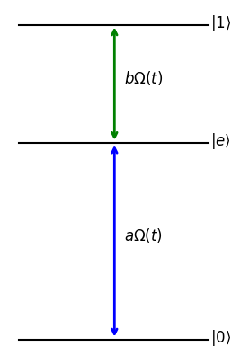
\(|0\rangle\) and \(|1\rangle\) evolve to states:
and
By keeping the ratio between \(a/b\) constant, the evolution satisfies
If the pulse length \(\tau\) is such that \(\int_0^\tau \Omega(t) dt = 2\pi\) then the operator acting on \(span[|0\rangle, |1\rangle]\) is:
where \(e^{i\phi}\tan\theta/2 = a/b\)
def U_C(theta, phi=0):
return np.array([[np.cos(theta), np.exp(1j * phi) * np.sin(theta)],
[np.exp(-1j * phi) * np.sin(theta), -np.cos(theta)]])
def get_a_b(theta, phi=0, a=1):
left = np.exp(1j * phi) * np.tan(theta/2)
b = a / left
norm = np.sqrt(np.abs(a)**2 + np.abs(b)**2)
return (a/norm, b/norm)
res = 100
t = np.linspace(-3, +3, res)
sigma = 0.01
ip = np.exp((-.5* sigma**2) * t ** 2)
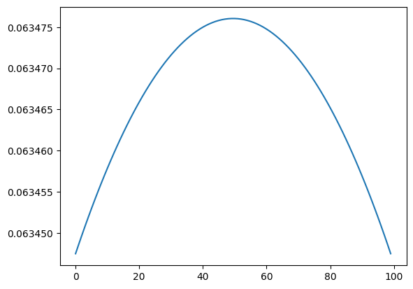
gaussian_pulse = 2*np.pi / np.trapz(ip) * ip
print(f"Integral: {np.trapz(gaussian_pulse)}")
plt.plot(gaussian_pulse)
plt.show()
Integral: 6.2831853071795845
theta = np.pi / 4
phi = np.pi

print(f"Expected Unitary:\n{U_C(theta)}")
Expected Unitary:
[[ 0.70710678+0.j  0.70710678+0.j]
 [ 0.70710678+0.j -0.70710678+0.j]]
ket_0 = np.array([[1],[0],[0]])
ket_e = np.array([[0],[1],[0]])
ket_1 = np.array([[0],[0],[1]])

a, b = get_a_b(theta, phi)

H = a * ket_e @ ket_0.conj().T + b * ket_e @ ket_1.conj().T
H = H + H.conj().T
t_range = np.linspace(0, res, res)
H_qobj = [0.5 * qp.Qobj(H), gaussian_pulse]
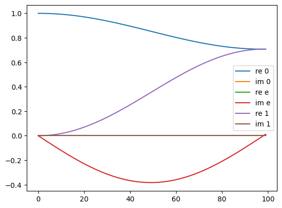
result = qp.mesolve(H_qobj, qp.Qobj(ket_0), t_range)
plt.plot([r.full()[0][0].real for r in result.states], label='re 0')
plt.plot([r.full()[0][0].imag for r in result.states], label='im 0')

plt.plot([r.full()[1][0].real for r in result.states], label='re e')
plt.plot([r.full()[1][0].imag for r in result.states], label='im e')

plt.plot([r.full()[2][0].real for r in result.states], label='re 1')
plt.plot([r.full()[2][0].imag for r in result.states], label='im 1')
plt.legend()
plt.show()
qubit_states = [r.eliminate_states([1]) for r in result.states]
bh = qp.Bloch()
bh.point_color = ['b']
bh.add_states(qubit_states, 'point')
bh.add_states([qubit_states[0], qubit_states[-1]])
bh.show()