Tomography#

Characterization is concerned with the following main question: what exactly did the quantum computer do? This may manifest in a few ways:

What is the state \(\rho\) of the quantum computer?
What is the operation \(\mathcal O\) that is being performed by the quantum computer?

How close is the quantum computer’s state to my state?
How accurate is my desired operation \(U\)?

State Tomography#

What is the state \(\rho\) of the quantum computer?

Let us introduce state tomography by walking through a simple qubit example.

Suppose we start in an arbitrary qubit density state, which we may write as:

\[ \rho = \frac{1}{2}(I + a_x\sigma_x + a_y\sigma_y + a_z\sigma_z) \]

where \(\vec{a}\) is a real number. So how would be figure out coefficients \(\vec{a}\)? Let us take a look at the expectation value of \(\sigma_x\):

\[\begin{split} \begin{align} \expectationvalue{\sigma_x} &= \mathrm{Tr} (\rho \sigma_x) \\ &= \frac{1}{2} \left( \mathrm{Tr}(I\sigma_x) + a_x \mathrm{Tr}(\sigma_x \sigma_x) + a_y \mathrm{Tr} (\sigma_y \sigma_x) + a_z \mathrm{Tr}(\sigma_z\sigma_x) \right) \\ &= \frac{1}{2} (a_x \cdot 2) = a_x \end{align} \end{split}\]

Note

For an observable \(M\), \(\expectationvalue{M} = \mathrm{Tr}(\rho M)\) and Pauli matrices follow the identity \(\mathrm{Tr}(\sigma_\alpha \sigma_\beta) = 2\delta_{\alpha,\beta}\)

We have shown that the expectation values of the Pauli matrices (same deduction for \(\sigma_y\) and \(\sigma_x\) as above) has a direct relation with the density matrix of the state. Therefore by computing the expectation values of an appropriate set of observables we can compute the density state.

Now, we can compute the expectation value by performed repeated measurements. We can project the state into each basis, repeating the experiment a large number of times, and using the resulting counts to get the expectation value.

Note

Given an observable \(M\), we can

(1)#\[\begin{split} \begin{align} \bra{\psi} M \ket{\psi} &= \bra{\psi} U^\dagger \Lambda U \ket{\psi} = \bra{\psi^\prime} \Lambda \ket{\psi^\prime} \\ &= \sum_i \braket{\psi^\prime}{i}\bra{i}\Lambda\ket{i}\braket{i}{\psi^\prime} = \sum_i \lambda_i |\bra{i}\ket{\psi^\prime}|^2 \end{align} \end{split}\]

Since \(M\) is Hermitian, we are able to diagonalize it by a unitary matrix \(U\) and a diagonal matrix with real entries \(\Lambda\) (corresponding to eigenvalues). We let the quantum computer perform the operation \(U\), and then measure in a standard basis, \(\ket{i}\). We can then recover the expectation value of \(M\) by multiplying the outcomes by the eigenvalues \(\lambda_i\).

TL;DR:

Expectation values of a set of observables let us deduce the density matrix

Through repeated measurements we can estimate the expectation values

Python Example#

Let us now walk for an example of performing state tomography on arbitrary dimensions. First, we are using liepy, a library that has convenience functions to generate various matrix groups.

import liepy as lp

For a \(d\)-dimensional quantum system, let use the generalized Gell-Mann matrices to create the set observables \(\{M\}\)

def qudit_tomography(d: int = 2) -> list[np.ndarray]:
    """
    Creates the Hermitian matrix basis for a single qudit.

    Parameters
    ----------
    d : int, optional
        Dimension of qudit, defaults to a qubit (d = 2)
    """
    basis = lp.gen_gellmann(d)
    basis = [-1j * b for b in basis]
    basis = [np.eye(d)] + basis
    return basis

We also create a function that simply computes the tensor basis for several qudits

def qudits_tomography(d: int = 2, n: int = 1) -> list[np.ndarray]:
    """
    Creates the Hermitian matrix basis for a single qudit.

    Parameters
    ----------
    d : int, optional
        Dimension of qudit, defaults to a qubit (d = 2)
    n : int
        Number of qudits
    """

    qudit_basis = qudit_tomography(d)
    tensors = product(qudit_basis, repeat=n)
    basis = []
    for t in tensors:
        tensor = reduce(lambda x, y: np.kron(x, y), t)
        basis.append(tensor)

    return basis

Now we create a class that holds information about the observables \(\{M\}\), but also computes the unitary operators following (1). We also define functions that (a) takes a set of probabilities (from an experiment) and converts them to expectation values (1), and (b) computes the density matrix from expectation values.

from itertools import product
from functools import reduce

class QuditTomography(object):
    def __init__(self, d: int = 2, n: int = 1):
        self.d = d
        self.n = n
        self.dim = d ** n
        self.basis = qudits_tomography(d, n)
        self.A = np.stack([b.flatten().conj() for b in self.basis])

        # Compute the Unitary operators for change-of-basis
        eigh = [np.linalg.eig(b) for b in self.basis]
        eigh = [*zip(*eigh)]
        self.eigs, self.Us = eigh

        # Need to diagonalize such that U^dag L U = H
        # but default numpy is U L U^dag = H
        # so we make U be the conjugate transpose
        self.Us = [u.conj().T for u in self.Us]

    def fit(self, probabilities: list[np.ndarray]):
        """
        Given the probabilities for each experiment, 
        compute the density matrix via linear inversion

        Parameters
        ----------
        probabilities: list[np.ndarray]
            A list of experiments' probability results
        """
        expectations = np.array([np.sum(e @ p)
                                for e, p in zip(self.eigs, probabilities)])
        return self.fit_expectations(expectations)

    def fit_expectations(self, expectations: np.ndarray):
        """
        Use linear inversion to fit a density matrix rho from expectation values

        Parameters
        ----------
        expectations: np.ndarray
            An array of expectation values
        """
        #expectations = np.atleast_2d(expectations[:]).T
        rho = np.linalg.pinv(self.A.T @ self.A) @ self.A.T @ expectations
        rho = rho.reshape(self.dim, self.dim)
        return rho

Fake experiment: a qubit#

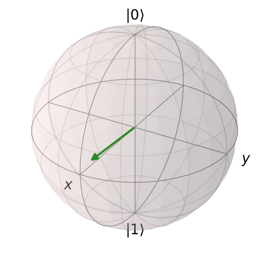
Suppose we have a random quantum state

rho = qp.rand_dm_hs(2)
print(rho.data)
b = qp.Bloch()
b.add_states(rho)
b.show()

  (0, 0)	(0.3949686129018373+0j)
  (0, 1)	(0.23936809063185968+0.11437042383096704j)
  (1, 0)	(0.23936809063185968-0.11437042383096704j)
  (1, 1)	(0.6050313870981627+0j)

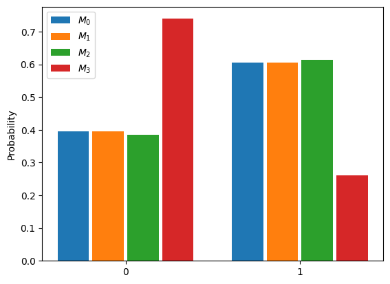
Let us recover it using quantum state tomography. First we compute the probabilities for the different observables

tomo = QuditTomography(2, 1)
Us = tomo.Us

rho = rho.data.toarray()

states = []
for U in Us:
    state = U @ rho @ U.conj().T
    states.append(state)

# define projection operators in the standard basis
P = [np.array([[1, 0], [0, 0]]), np.array([[0, 0], [0, 1]])]

# compute the probabilites after basis transformation
probabilities = [[np.trace(state @ p).real for p in P] for state in states]

labels = ['0', '1']

data = {r"$M_{}$".format(i): p for i, p in enumerate(probabilities)}
fig, ax = plt.subplots()
bar_plot(ax, data, total_width=.8, single_width=.9)
ax.set_xticks(range(2), ["0", "1"])
plt.ylabel("Probability")

plt.show()

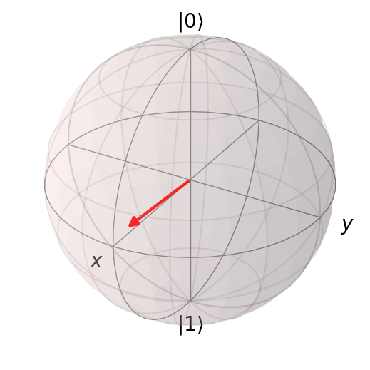
Now let us reconstruct the state from these probabilities

rho_r = tomo.fit(probabilities)

b = qp.Bloch()
b.vector_color = ['r']
b.add_states(qp.Qobj(rho_r))
b.show()

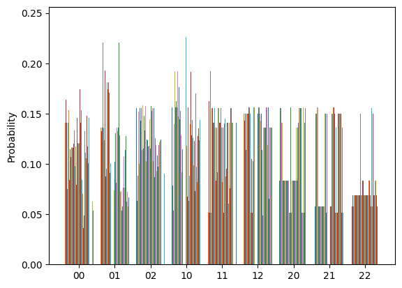
Fake experiment: two qutrits#

d = 3
n = 2

rho = qp.rand_dm_hs(d**n)

tomo = QuditTomography(d, n)
Us = tomo.Us

rho = rho.data.toarray()

states = []
for U in Us:
    state = U @ rho @ U.conj().T
    states.append(state)

# define projection operators in the standard basis
basis = []
for d_i in range(d):
    b = np.zeros((d,d))
    b[d_i, d_i] = 1
    basis.append(b)
basis = product(basis, repeat=n)
P = []
for t in basis:
    p = reduce(lambda x, y: np.kron(x, y), t)
    P.append(p)


# compute the probabilites after basis transformation
probabilities = [[np.trace(state @ p).real for p in P] for state in states]

labels = ['0', '1', '2']
labels = [x[0] + x[1] for x in product(labels, repeat=n)]

data = {r"$M_{}$".format(i): p for i, p in enumerate(probabilities)}
fig, ax = plt.subplots()
bar_plot(ax, data, total_width=.8, single_width=.9, legend=False)
ax.set_xticks(range(d**n), labels)
plt.ylabel("Probability")

plt.show()

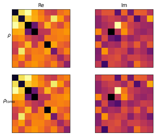
rho_r = tomo.fit(probabilities)

print(f"Is our fitted state close to original? {np.allclose(rho_r, rho)}")

Is our fitted state close to original? True

fig, axes = plt.subplots(nrows=2, ncols=2, sharey=True, sharex=True)

im = axes[0, 0].matshow(rho.real, cmap=plt.cm.inferno_r)
im = axes[0, 1].matshow(rho.imag, cmap=plt.cm.inferno_r)

im = axes[1, 0].matshow(rho_r.real, cmap=plt.cm.inferno_r)
im = axes[1, 1].matshow(rho_r.imag, cmap=plt.cm.inferno_r)

plt.setp(plt.gcf().get_axes(), xticks=[], yticks=[]);

axes[0, 0].set_ylabel(r"$\rho$", rotation=0, size='large')
axes[1, 0].set_ylabel(r"$\rho_\mathrm{tomo}$", rotation=0, size='large')

axes[0, 0].set_title("Re", size='large')
axes[0, 1].set_title("Im", size='large')

fig.tight_layout()

Drawbacks#

Quantum state tomography does come with several drawbacks. Examples include:

We need to perform a unitary operator to change the basis, this operator may be noisy and not faithfully change the basis.
The actual results of measurement may be inaccurate, biasing the result
We are cursed by dimensionality: with higher number of dimensions we need higher probabilistic accuracy and therefore need more experiment repetitions + measurements.

Many works introduce methods to overcome these drawbacks, such as:

Process Tomography#

What is the operation \(\mathcal O\) that is being performed by the quantum computer?

The previous section described strategies to recover a state \(\rho\) from a quantum system. This section discusses strategies for recovering a quantum operation acted onto a state. Namely, the goal is to find the underlying process that the quantum system undertook. As an example, let us ask the quantum computer to perform the Hadamard gate:

\[\begin{split} H = \frac{1}{\sqrt{2}} \begin{bmatrix} 1 & 1 \\ 1 & -1 \end{bmatrix}. \end{split}\]

We would like to test if the quantum computer actually performs the Hadamard gate; perhaps there is noise that modifies the effective gate operation. In general, any physical operation to a quantum state \(\rho\) can be described by a completely positive map

\[ \mathcal{E}(\rho) = \sum_i K_i \rho K_i^\dagger \]

where \(K_i\) are operation elements and must satisfy \(\sum_i K_i^\dagger K_i \leq I\) so that \(\Tr[\mathcal{E}(\rho)] \leq 1\). By writing the operators \(K_i\) in terms of an orthogonal basis \(\{E_i\}\) endowed with the Hilbert-Schmidt inner product

\[ K_i = \sum_m a_{im} E_m \]

we then have

\[ \mathcal{E}(\rho) = \sum_{m,n} \chi_{mn} E_m \rho E_n^\dagger, \quad \chi_{mn} = \sum_i a_{mi} a^*_{ni}. \]

Hence, the goal of quantum process tomography is to solve for the superoperator \(\chi\) which characterizes the process \(\mathcal{E}\) with respect to the \(\{E_i\}\) basis. Continuing the simple example of a quantum computer implementing the Hadamard gate, let the basis consist of the normalized Pauli matrices \(\{I, X, Y, Z\}/\sqrt{2}\) then the coordinates in this basis for the Hadamard matrix are \((0, -i, 0, -i)\). Hence

\[\begin{split} \chi = \begin{bmatrix} 0 & 0 & 0 & 0\\ 0 & 1 & 0 & 1\\ 0 & 0 & 0 & 0\\ 0 & 1 & 0 & 1\\ \end{bmatrix} \end{split}\]

Standard Approach#

As implied in the previous section, a standard approach to quantum process tomography is to take each element of a linearly independent set and send it through the process, followed by quantum state tomography.

Namely,

Start with \(d^2\) (for qubits \(d=2^n\)) linearly independent inputs \(\rho_i\)
Obtain \(\mathcal{\rho_i}\) by sending it through the process
Perform quantum state tomography to determine \(c_{i,j}\) where \(\mathcal{\rho_i} = \sum_j c_{i,j}\rho_j\)
Solve a linear equation (matrix inversion) to obtain \(\chi\)

Real experiments on one-or-two qubits often use this approach. But such an approach takes on the weaknesses of quantum state tomography, and in addition introduces complexity such as requiring initialization of \(d^2\). For a complete approach, the standard quantum process tomography will require \({2^n}^2 \cdot ({2^n}^2 -1)\) basis measurements.

Quantum Noise Characterization and Mitigation

Tomography

Contents

Tomography#

State Tomography#

Python Example#

Fake experiment: a qubit#

Fake experiment: two qutrits#

Drawbacks#

Process Tomography#

Standard Approach#