Pulse Optimization

Optimal control theory is an extremely versatile set of techniques that can be applied in many situations. Although optimal control entails many fields, the general idea is to use a feedback loop between an agent and a target system. Optimal control is applied to several quantum technologies, including the pulse shaping of gate designs in quantum circuits to minimize noise. Generally, the pulse shaping is a passive technique, whereby a classically computation takes place beforehand to find an optimal pulse without active feedback from a quantum system }. Gradient Ascent Pulse Engineering (GRAPE) is a powerful technique that uses gradient ascent and a nonlinear optimization solver, such as Broyden–Fletcher–Goldfarb–Shanno (BFGS) algorithm, to solve for a pulse shape to achieve a desired operation. Although powerful, the technique requires the simulation of quantum dynamics on a classical computer, which scales exponentially with quantum system size.

Quantum optimal control deals with fitting pulses \(a_i(t)\), or \(a_{i,n}\) for a discrete solution, for a Hamiltonian \(H\) oftern written written in terms of a drift \(H_d\) and several control Hamiltonians \(H_{i}\) that are modulated by pulses. The dynamics is governed by

\[ \pdv{}{t}\ket{\psi} = \left(H_d + \sum_i a_i(t)H_{i} \right)\ket{\psi}. \]

Many factors play into the quality of pulses, including time, amplitude, shape, as well as hardware-specific limitations in sampling rate.

Python Example

import qutip as qp

T = 1
times = np.linspace(0, T, 100)


H = np.array([[1, 1], [1, -1]]) / np.sqrt(2)

H0 = 0 * np.pi * qp.sigmaz()


R = 150
H_ops = [qp.sigmax(), qp.sigmay()]

from qutip.control import cy_grape_unitary
from qutip.ui.progressbar import TextProgressBar

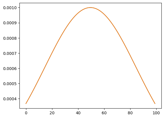
x = np.linspace(-1, +1, times.size)
initial_amplitudes = 1e-3 * np.stack([np.exp(-x**2), np.exp(-x**2)], -1)

qutip_pulse = cy_grape_unitary(qp.Qobj(H), H0, H_ops, R, times,u_start=initial_amplitudes.T, eps=2*np.pi/T, phase_sensitive=False)

plt.plot(initial_amplitudes)
plt.show()

qutip_pulse.u.shape
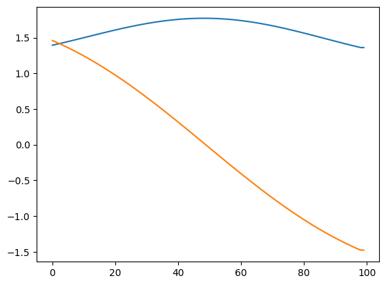
plt.plot(qutip_pulse.u[-1, 0,:])
plt.plot(qutip_pulse.u[-1, 1,:])
plt.show()

psi0 = qp.basis(2, 0)
c_ops = []
e_ops = [qp.sigmax(), qp.sigmay(), qp.sigmaz()]

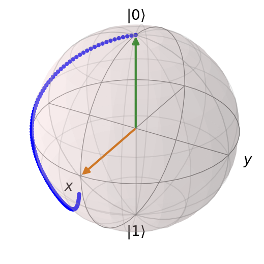
result = qp.mesolve(qutip_pulse.H_t, psi0, times, c_ops, e_ops)

b = qp.Bloch()
b.add_points(result.expect)

b.add_states(psi0)
b.add_states(qp.Qobj(H) * psi0)
b.show()

Holonomic Quantum Computing

Holonomic quantum computing exploits the notion of parallel transport. Consider, for example, a vector that is transported around in a closed loop along a sphere – as shown in figure~\ref{fig:parallel-transport}. It turns out that the vector itself will rotate by angle \(\alpha\), dependent on the total area covered by the closed loop. As long as the area remains the same, the actual path does not matter. Holonomic quantum computing exploits this principle to produce gates that are robust to noise in the control path. Namely, it can produce a propogator \(U\) that is factorized into two terms, \(U = V(T) \otimes \Gamma\) where \(V(T)\) is the dynamical part, and \(\Gamma\) is a unitary transformation which is determined only by the geometry of the quantum system and is called geometric phase. We then recall that the geometric factor can be discussed in the case of Abelian U\((1)\) and non-Abelian U\((N)\) phase factors.

Consider a time-dependent Hamiltonian \(H(t)\), with a solution to the corresponding Shrödinger equation \(\ket{\psi(t)}\) in a time window \(t \in [0, T]\). The solution of the Schrödinger equation

\[ i \dv{}{t} \ket{\psi(t)} = H(t) \ket{\psi(t)} \]

defines a curve

\[ C : t \in [0, T] \longrightarrow \ket{\psi(t)} \in \mathcal{H}. \]

Taking a representative \(\ket{\phi(t)}\) along the curve, it is related to the solution via a local phase transformation

\[ \ket{\psi(t)} = e^{i\chi(t)} \ket{\phi(t)} \]

We can rewrite the previous equation as:

\[ i \dv{}{t} \left [ e^{i\chi(t)} \ket{\phi(t)} \right ] = e^{i\chi(t)} H(t) \ket{\phi(t)}, \]

and

\[ -\dot\chi(t)e^{i\chi(t)}\ket{\phi(t)} + ie^{i\chi(t)}\ket{\dot\phi(t)} = e^{i \chi(t)}H(t)\ket{\phi(t)}. \]

Multiplying \(\bra{\psi(t)}\) on the left, we have

\[ \dot\chi(t) = i\bra{\phi(t)}\ket{\dot\phi(t)} - \bra{\phi(t)}H(t)\ket{\phi(t)}, \]

which yields

\[ \chi(T) - \chi(0) = \int_0^T i\bra{\phi(t)}\ket{\dot\phi(t)} - \int_0^T \bra{\phi(t)}H(t)\ket{\phi(t)}. \]

The first term on on the right hand side is invariant under time parametrization \(t \rightarrow t^\prime(t)\) and can be written as \(\int i \bra{\phi}\ket{d\phi}\). The second term is invariant under phase transformations \(\ket{\chi(t)} \rightarrow e^{i\alpha}\ket{\phi(t)}\), but not under time parametrization. This term is the instantaneous expectation value of the energy \(E(t)\) computing along the solution. The yields a final equation:

\[ \chi(T) - \chi(0) = - \int_{\phi(t)} A - \int_{\phi(t)} E(t)dt \]

A special cases occurs when the evolution of the system is cyclic, i.e. \(\ket{\phi(T)} = e^{i\alpha} \ket{\psi(0)}\). Selecting a representative closed curve \(\ket{\phi(t)}\), with \(\ket{\phi(t)} = e^{i \chi(t)}\ket{\phi(t)}\) and \(\ket{\phi(T)} = \ket{\phi(0)} = \ket{\psi(0)}\) we have that

\[ \alpha = - \oint_{\phi(t)} A - \oint_{\phi(t)} E(t) dt \]

Note that for a closed curve, the integral \(\oint A\) is invariant. The corresponding phase factor \(e^{i \oint A}\) is called the holonomy.

Take a coherent superposition of the initial and final state

\[ \ket{\psi(0)} + \ket{\psi(T)} = (1 + e^{i\alpha}) \ket{\psi(0)} \]

we can in principle observe an interference pattern which is made by two contributions: the dynamical phase which is given by the instantaneous energy as \(\oint E(t) dt\), and an additional phase shift which is the holonomy \(e^{-\oint A}\). Since the additional factor \(e^{-i\oint A}\) only depends on the loop, it is called the geometric phase. Since the cyclic dynamics appear as a special feature for the solution of the Schrodinger equation, it can only be determined a posteriori, and, in general, the time dependence of the Hamiltonian does not given any information about it, e.g. the Hamiltonian might not be cyclic, \(H(T) \neq H(0)\).

However, finding holonomic gates in state space is abstract. In an experimental setting, there is no direct handling of quantum states, rather the only information is the effective Hamiltonians that drive a system. It would be preferable to control a system and determine a priori if the evolution of the system will be cyclic. One way this can be done is by working in the adiabatic regime, which places a requirement in the rate of change of a Hamiltonian. Alternatively, one can ignore the adiabatic constraint, but work with systems which have an effective Hamiltonian that provides some sort of known guarantee of cyclic evolution.

Consider a quantum system with a finite number of levels, \(\mathcal{H} \cong \mathcal{C}^N\). The Hamiltonian can be written as

\[ H = \sum_\alpha h_\alpha \lambda_\alpha \]

where \(h_\alpha\) is a real and the operators \(\{\lambda_\alpha\}_{\alpha=1}^{N^2}\) are a basis in the linear space of Hermitian operators, such as the generalized Gell-Mann matrices, or the Pauli matrices for \(N = 2\). From this point of view, a Hamiltonian is an element in a \(N^2\)-dimensional real vector space. Hence, a time dependent Hamiltonian,

\[ H(t) = \sum_\alpha h_\alpha(t) \lambda_\alpha \]

defines a path in \(\mathcal{R}^{N^2}\), and a cyclic Hamiltonian a closed loop. However, the emphasis here is that the quantum state must be cyclic in order to realize a holonomy, and not necessarily the Hamiltonian. In the adiabatic regime, we can say that a cyclic Hamiltonian will result in a cyclic state, but this is not always true.